
Swimlane heatmap for longitudinal trajectories
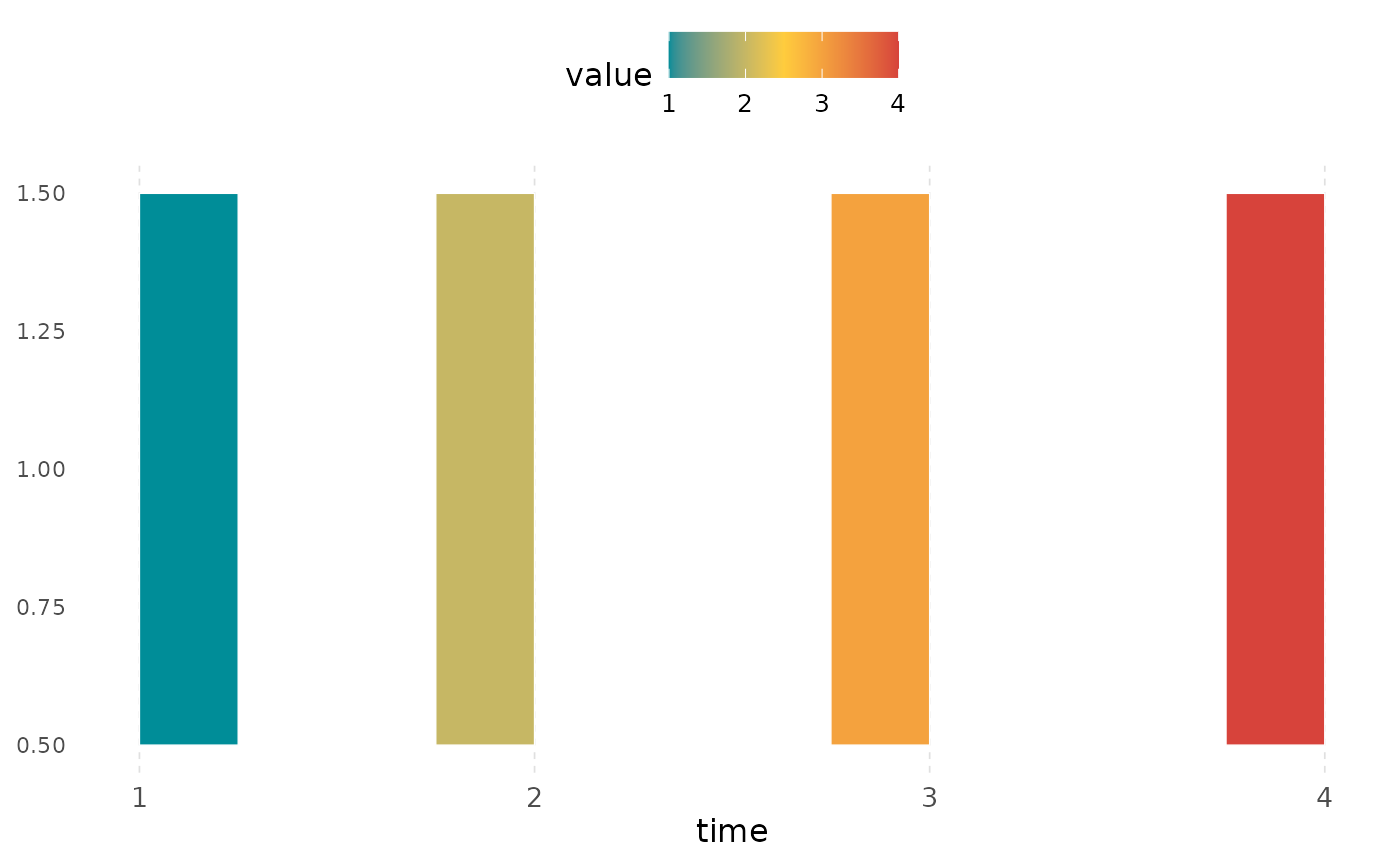
geom_kodom_heatmap.RdDivides the time axis into equal-width bins and fills each (subject × bin) cell with an aggregate of the measured value. Each subject occupies one horizontal lane. Use this layout when the cohort is large or when you prefer a compact, aligned grid over individual paths.
Usage
geom_kodom_heatmap(
  mapping = NULL,
  data = NULL,
  stat = StatKodomHeatmap,
  position = "identity",
  ...,
  sort_by = "mean",
  n_max = Inf,
  bins = 10L,
  breaks = NULL,
  fun = "mean",
  na.rm = FALSE,
  show.legend = NA,
  inherit.aes = TRUE
)
Arguments
- mapping
Set of aesthetic mappings created by
ggplot2::aes().- data
A data frame. If
NULL, inherits from the plot.- stat
The stat to use. Defaults to StatKodomHeatmap.
- position
Position adjustment, almost always
"identity".- ...
Other arguments passed to
ggplot2::layer().- sort_by
Lane ordering. One of
"none","mean"(default),"mean_asc","first","last"— all refer to thefillvariable.- n_max
Maximum number of subjects to display. A random sample is taken when exceeded. Default
Inf(all subjects).- bins
Number of equal-width time bins. Default
10L. Ignored ifbreaksis supplied.- breaks
Numeric vector of explicit bin boundaries. Overrides
bins.- fun
Aggregation function per cell. One of
"mean"(default),"median","first","last","min","max".- na.rm
If
TRUE, silently remove rows with missing required aesthetics.- show.legend
Logical. Should this layer appear in the legend?
- inherit.aes
If
FALSE, overrides the default aesthetics.
Details
Lane ordering is controlled by sort_by (defaults to "mean", which
places the highest-mean subjects at the top). Time bins can be
customised via bins (number of equal-width intervals) or breaks
(explicit boundaries).
Aesthetics
Required aesthetics are shown in bold.
x— time variable (numeric or Date)id— subject identifier; determines lane position on the y axisfill— measurement value used for cell color and sortingcolour— tile border color (default"white")linewidth— tile border width (default0.25)alpha— transparency
Examples
# \donttest{
library(ggplot2)
df <- data.frame(
subject_id = rep(1:5, each = 4),
time = rep(1:4, 5),
visit_month = rep(1:4, 5),
value = rep(1:4, 5),
hba1c = rep(1:4, 5),
arm = rep(c("Treatment", "Control"), c(12, 8))
)
ggplot(df, aes(x = time, id = subject_id, fill = hba1c)) +
geom_kodom_heatmap(sort_by = "mean", bins = 12) +
scale_fill_kodom() +
theme_kodom()
 # }
# }