Counterfactual Trajectories with geom_kodom_branch

geom_kodom_branch() extends the swimlane layout with counterfactual prediction arms. Each subject has one observed trajectory (solid line) and one dashed sub-lane per medication or intervention arm, stacked vertically within the subject’s primary lane. The branch point can differ across subjects — just supply NA in the medication aesthetic for every pre-branch and post-branch observed row, and a non-NA arm label for every predicted row.

---

Sample data

The dataset simulates 8 patients from a diabetes trial. Each patient has pre-randomisation HbA1c readings (observed, medication = NA), a continued post-randomisation observed path, and model-predicted trajectories under two drug arms ("DrugA" and "DrugB"). Branch (randomisation) timing differs across patients.

set.seed(21)

n_patients <- 8L
branch_times <- c(4, 6, 4, 8, 6, 4, 6, 8) # month of randomisation
horizon <- 18L # last prediction month

make_patient <- function(i) {
  t_branch <- branch_times[i]
  base <- rnorm(1, mean = 8.0, sd = 0.8)

  # Pre-branch observed visits (every 2 months, including month 0)
  t_pre <- seq(0, t_branch, by = 2)
  v_pre <- base + cumsum(c(0, rnorm(length(t_pre) - 1L, -0.1, 0.25)))

  # Post-branch observed (patient actually received DrugA)
  t_post <- seq(t_branch + 2, horizon, by = 2)
  v_post <- tail(v_pre, 1L) + cumsum(rnorm(length(t_post), -0.18, 0.2))

  # Predictions under DrugA (steeper decline)
  v_a <- tail(v_pre, 1L) + cumsum(rep(-0.20, length(t_post))) +
    rnorm(length(t_post), 0, 0.1)

  # Predictions under DrugB (milder decline)
  v_b <- tail(v_pre, 1L) + cumsum(rep(-0.10, length(t_post))) +
    rnorm(length(t_post), 0, 0.1)

  rbind(
    data.frame(
      subject_id = sprintf("P%02d", i),
      month = t_pre,
      hba1c = pmax(5, v_pre),
      medication = NA_character_,
      stringsAsFactors = FALSE
    ),
    data.frame(
      subject_id = sprintf("P%02d", i),
      month = t_post,
      hba1c = pmax(5, v_post),
      medication = NA_character_,
      stringsAsFactors = FALSE
    ),
    data.frame(
      subject_id = sprintf("P%02d", i),
      month = t_post,
      hba1c = pmax(5, v_a),
      medication = "DrugA",
      stringsAsFactors = FALSE
    ),
    data.frame(
      subject_id = sprintf("P%02d", i),
      month = t_post,
      hba1c = pmax(5, v_b),
      medication = "DrugB",
      stringsAsFactors = FALSE
    )
  )
}

trial_df <- do.call(rbind, lapply(seq_len(n_patients), make_patient))

---

1. Basic usage

Map x to time, id to subject, colour to the measurement, and medication to the arm column. Observed rows (medication = NA) are automatically labelled "observed" in the stat output, so scale_linetype_manual() can target all three track types by name. A short vertical fork connector is drawn at each subject’s branch point.

ggplot(
  trial_df,
  aes(
    x          = month,
    id         = subject_id,
    colour     = hba1c,
    linetype   = medication,
    medication = medication
  )
) +
  geom_kodom_branch() +
  scale_x_continuous(breaks = seq(0, 18, by = 3)) +
  scale_linetype_manual(
    values = c("observed" = "solid", "DrugA" = "dashed", "DrugB" = "dotted")
  ) +
  scale_colour_kodom(name = "HbA1c (%)") +
  theme_kodom() +
  labs(title = "Observed trajectories with DrugA / DrugB predictions")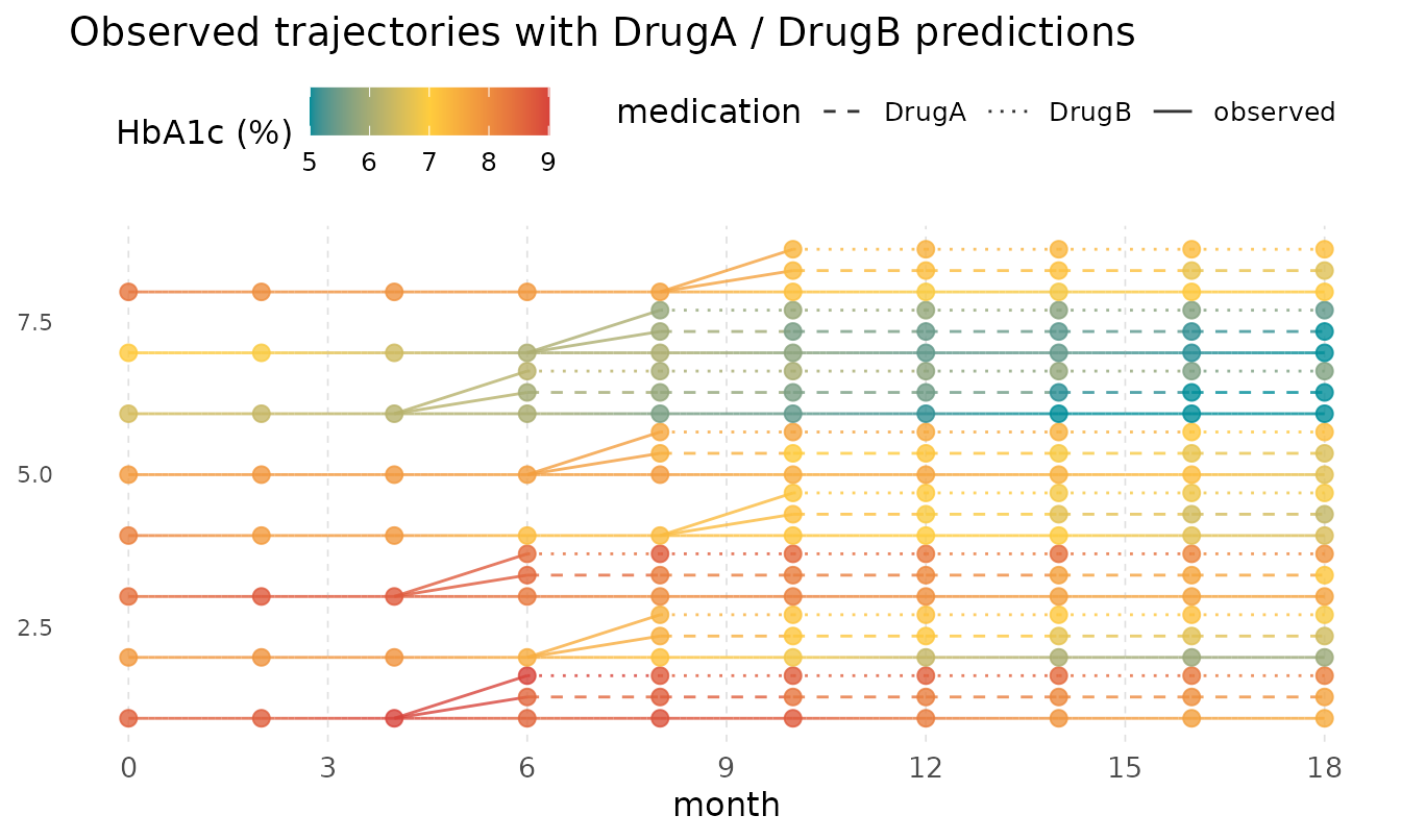

---

2. Controlling lane width and branch fraction

lane_width sets the vertical distance between subjects — increase it when lanes feel crowded. branch_fraction controls how much of that space the prediction sub-lanes occupy: with branch_fraction = 0.6 and two arms, each arm sits 0.30 * lane_width above the observed path.

ggplot(
  trial_df,
  aes(
    x          = month,
    id         = subject_id,
    colour     = hba1c,
    linetype   = medication,
    medication = medication
  )
) +
  geom_kodom_branch(lane_width = 2, branch_fraction = 0.6) +
  scale_x_continuous(breaks = seq(0, 18, by = 3)) +
  scale_linetype_manual(
    values = c("observed" = "solid", "DrugA" = "dashed", "DrugB" = "dotted")
  ) +
  scale_colour_kodom(name = "HbA1c (%)") +
  theme_kodom() +
  labs(title = "Wider lanes (lane_width = 2), tighter branches (0.6)")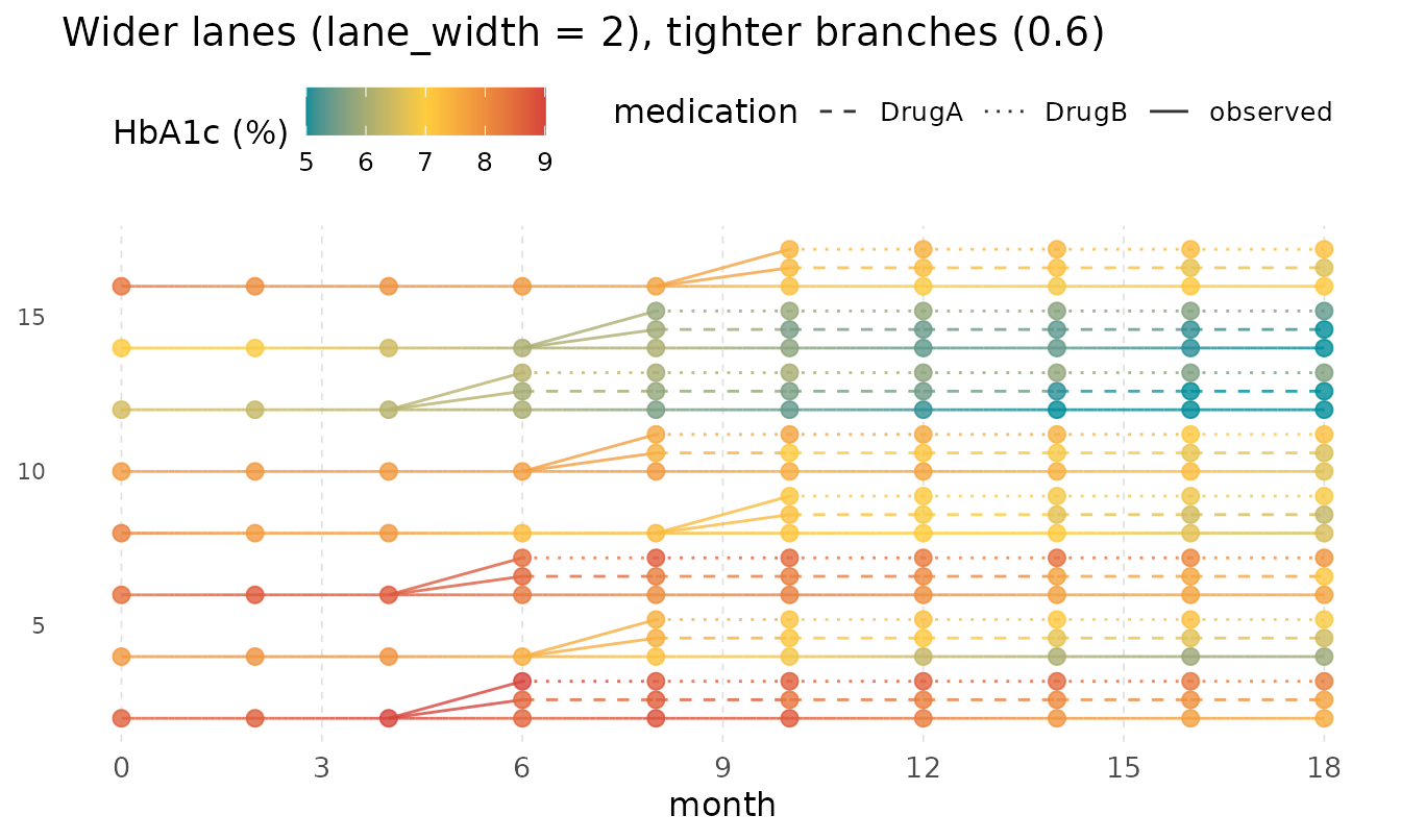

---

3. Lane ordering

sort_by controls the vertical order of subjects, using the colour variable as the sort key. "mean" places the highest-average subject at the top (smallest lane index); "mean_asc" reverses this.

ggplot(
  trial_df,
  aes(
    x          = month,
    id         = subject_id,
    colour     = hba1c,
    linetype   = medication,
    medication = medication
  )
) +
  geom_kodom_branch(lane_width = 2, sort_by = "mean") +
  scale_x_continuous(breaks = seq(0, 18, by = 3)) +
  scale_linetype_manual(
    values = c("observed" = "solid", "DrugA" = "dashed", "DrugB" = "dotted")
  ) +
  scale_colour_kodom(name = "HbA1c (%)") +
  theme_kodom() +
  labs(title = 'sort_by = "mean": highest average HbA1c at top')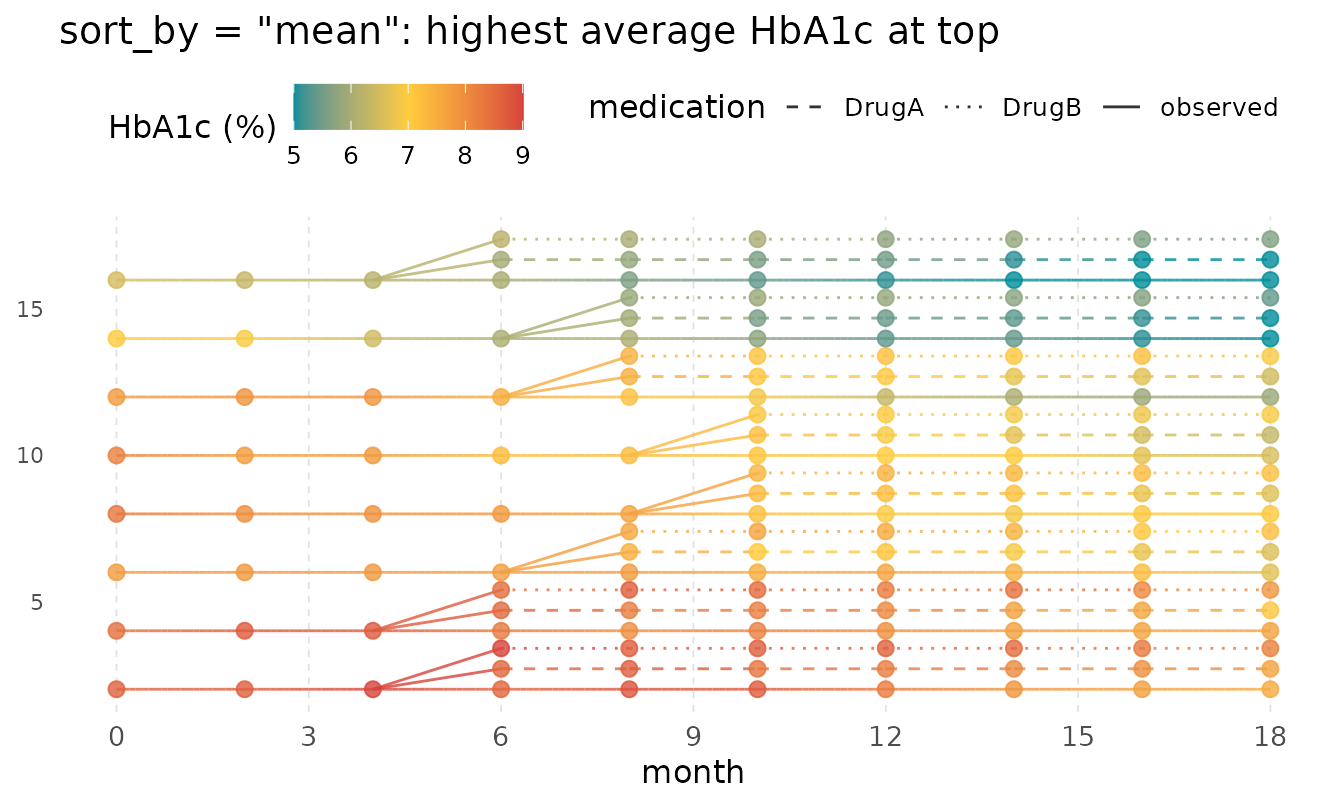

---

4. Labeling subjects on the y-axis

Because y is a real-valued lane position rather than a factor, ggplot2 shows numeric tick marks by default. Replace them with subject IDs by computing the break positions: with lane_width = lw, subject k sits at y = k * lw.

lw <- 2
patient_ids <- sort(unique(trial_df$subject_id))
n_pts <- length(patient_ids)

ggplot(
  trial_df,
  aes(
    x          = month,
    id         = subject_id,
    colour     = hba1c,
    linetype   = medication,
    medication = medication
  )
) +
  geom_kodom_branch(lane_width = lw, sort_by = "none") +
  scale_x_continuous(breaks = seq(0, 18, by = 3)) +
  scale_y_continuous(
    breaks = seq_len(n_pts) * lw,
    labels = patient_ids
  ) +
  scale_linetype_manual(
    values = c("observed" = "solid", "DrugA" = "dashed", "DrugB" = "dotted")
  ) +
  scale_colour_kodom(name = "HbA1c (%)") +
  theme_kodom() +
  labs(title = "Patient IDs on the y-axis", y = NULL)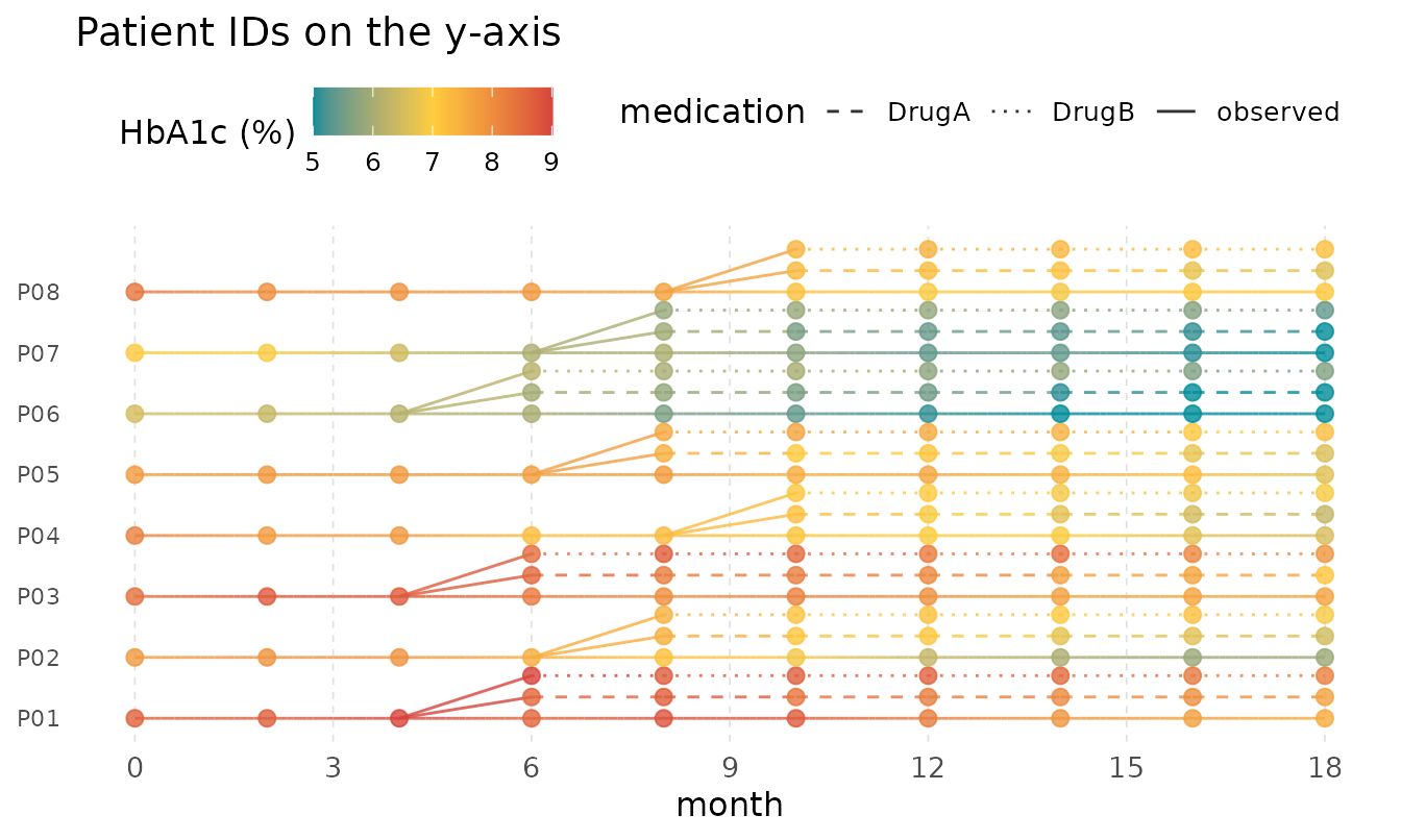

---

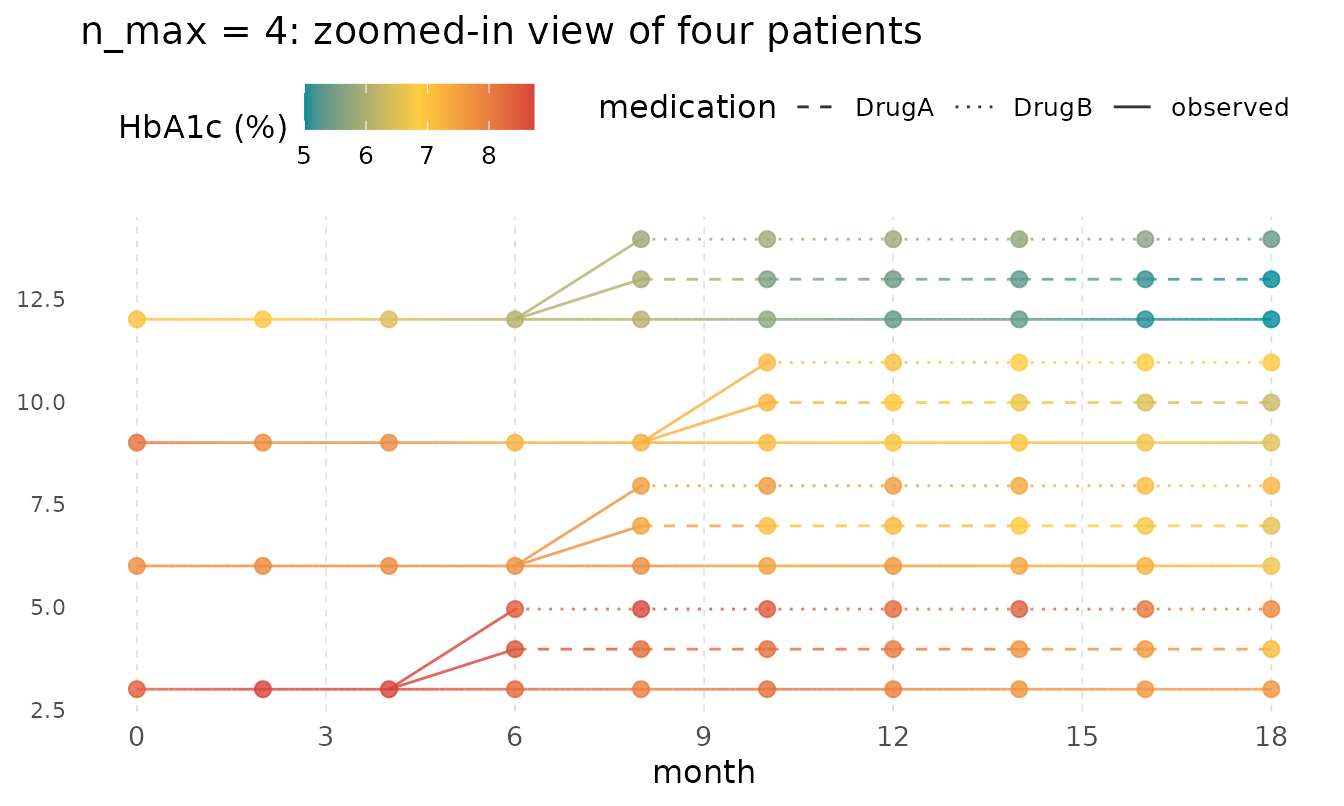
5. Subset with n_max

Pass n_max to focus on a random subset of subjects. Pair with a larger lane_width so each subject’s solid + dashed tracks are clearly readable.

ggplot(
  trial_df,
  aes(
    x          = month,
    id         = subject_id,
    colour     = hba1c,
    linetype   = medication,
    medication = medication
  )
) +
  geom_kodom_branch(
    n_max = 4L, lane_width = 3, branch_fraction = 0.65,
    sort_by = "mean"
  ) +
  scale_x_continuous(breaks = seq(0, 18, by = 3)) +
  scale_linetype_manual(
    values = c("observed" = "solid", "DrugA" = "dashed", "DrugB" = "dotted")
  ) +
  scale_colour_kodom(name = "HbA1c (%)") +
  theme_kodom() +
  labs(title = "n_max = 4: zoomed-in view of four patients")