
Kodom color scale for the color aesthetic
scale_color_kodom.RdA ggplot2 color scale using the Kadam flower palette (teal -> gold -> red).
Designed to compose with geom_kodom_line(), geom_kodom_heatmap(), and
geom_kodom_circular().
Usage
scale_color_kodom(
  colors = kodom_colors(),
  color_breaks = NULL,
  name = ggplot2::waiver(),
  discretize = FALSE,
  ...
)

scale_colour_kodom(
  colors = kodom_colors(),
  color_breaks = NULL,
  name = ggplot2::waiver(),
  discretize = FALSE,
  ...
)
Arguments
- colors
Color vector. Defaults to
kodom_colors().- color_breaks
Numeric breakpoints anchoring the gradient via
scales::rescale(). Fordiscretize = TRUE, each break adds one band:kbreaks producek + 1bands.NULL= evenly spaced.- name
Legend title. Defaults to
"value".- discretize
FALSE(default) = smooth gradient;TRUE= step bands atcolor_breaks.- ...
Ignored.
Details
Set discretize = TRUE to switch from a smooth gradient to solid color
bands separated at color_breaks — useful when values change slowly and
a continuous gradient washes out into a single hue.
Examples
# \donttest{
library(ggplot2)
df <- data.frame(
subject_id = rep(1:5, each = 4),
time = rep(1:4, 5),
visit_month = rep(1:4, 5),
value = rep(1:4, 5),
hba1c = rep(1:4, 5),
arm = rep(c("Treatment", "Control"), c(12, 8))
)
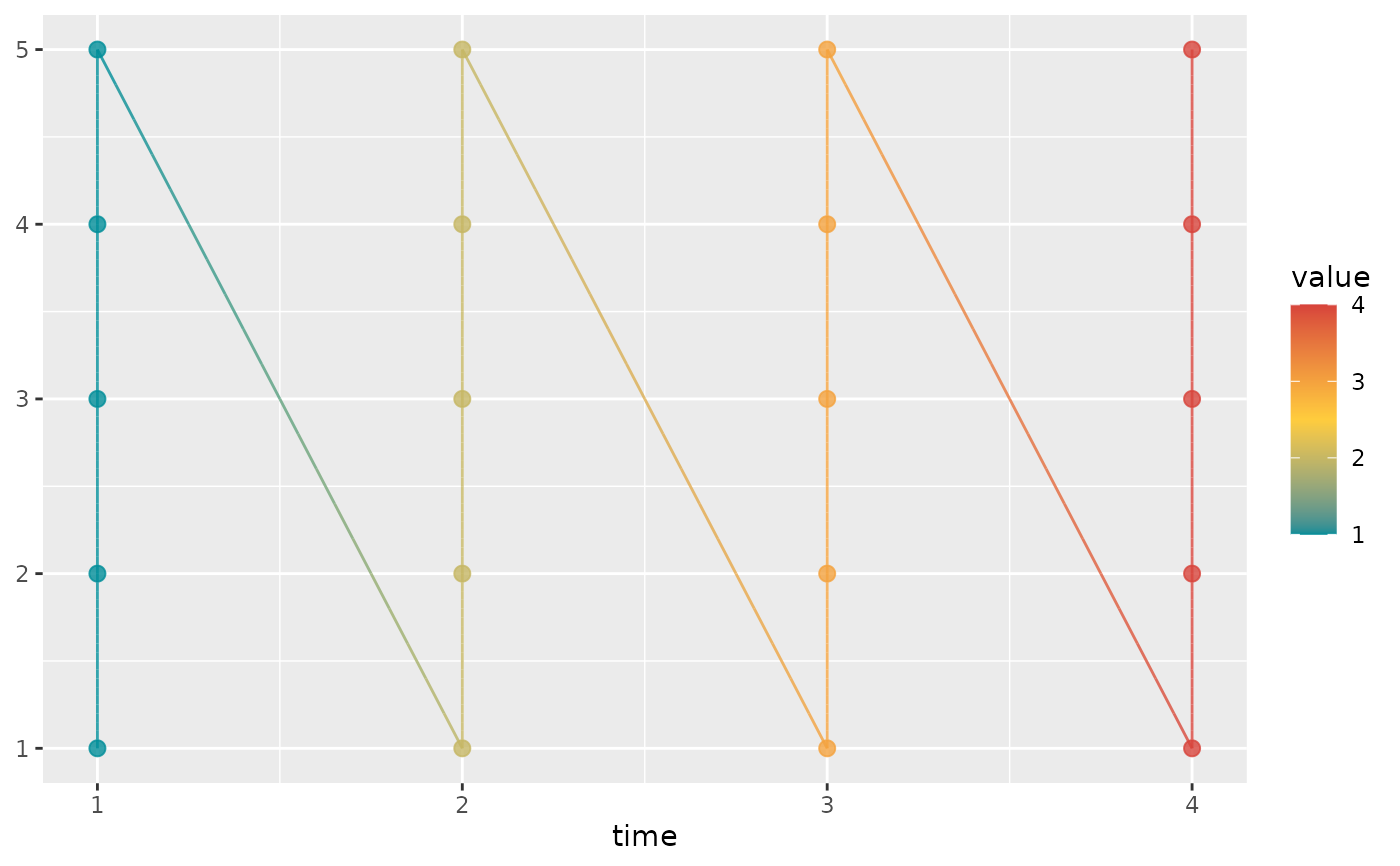
ggplot(df, aes(x = time, id = subject_id, color = value)) +
geom_kodom_line() +
scale_color_kodom()
 # Discrete bands at clinical thresholds
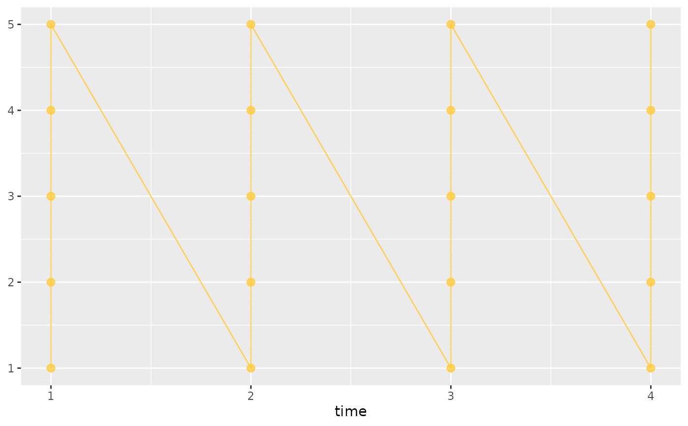
ggplot(df, aes(x = time, id = subject_id, color = hba1c)) +
geom_kodom_line() +
scale_color_kodom(discretize = TRUE, color_breaks = c(5.7, 6.5))
# Discrete bands at clinical thresholds
ggplot(df, aes(x = time, id = subject_id, color = hba1c)) +
geom_kodom_line() +
scale_color_kodom(discretize = TRUE, color_breaks = c(5.7, 6.5))
 # }
# }